We provide Habitat and Barrier data on various lizard species (nominally, Blue-tongued Lizard). The data was collected from Darebin Creek in Melbourne, which runs between Preston and West Heidelberg. For analysis purposes, a interpatch distance of 200 metres is recommended for lizard connectivity assessments.
Details
We provide helper functions to load the raster and shapefile data. These are required due to how the raster and vector data are stored. These functions provide easy access to example raster and shapefile data included with the package:
example_habitat()Returns a raster of lizard habitat data.example_barrier_shp()Returns a shapefile of lizard barrier data as an SF object.example_barrier()Returns a raster of lizard barrier data.
Examples
library(terra)
# Load habitat raster
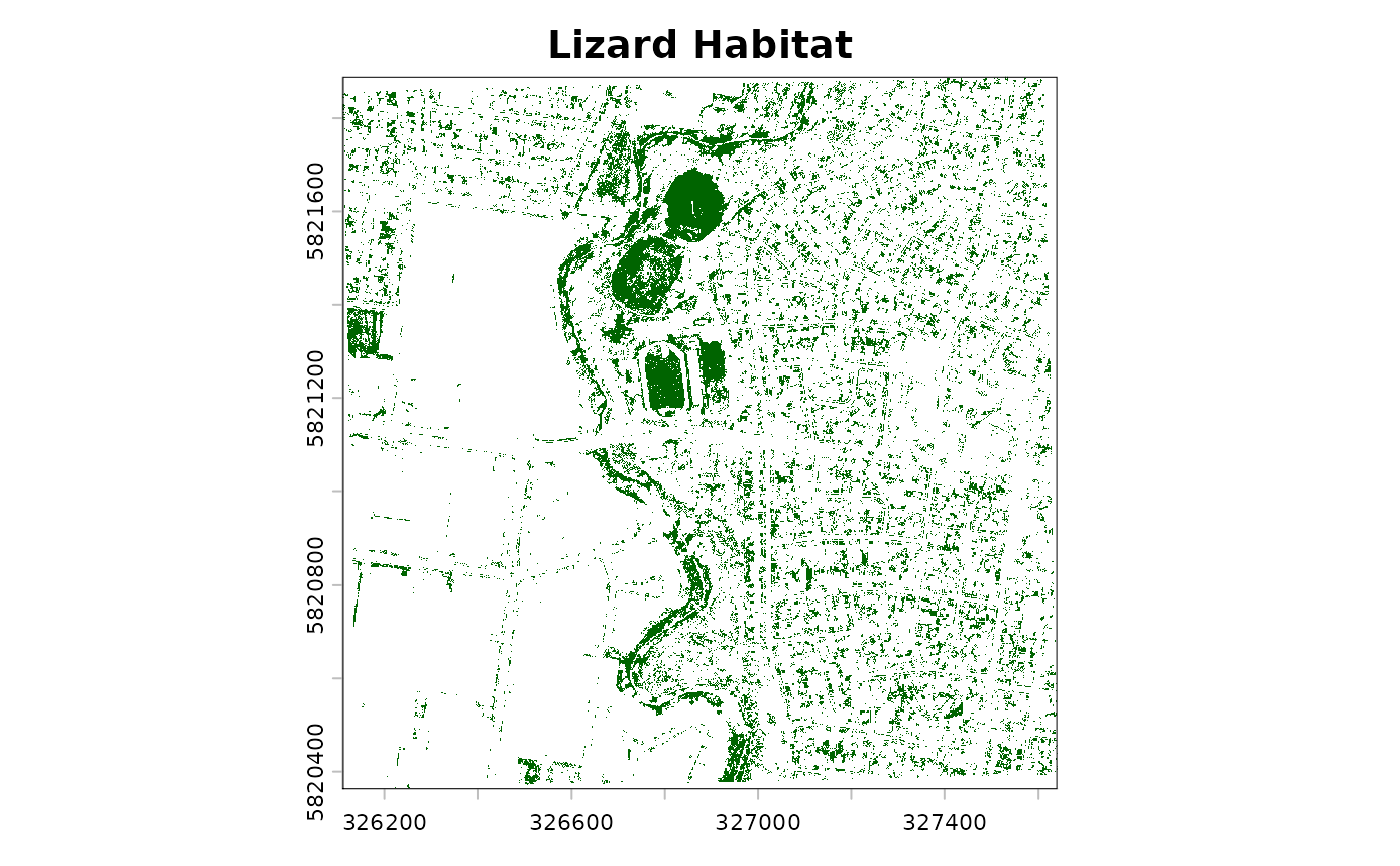
lizard_habitat <- example_habitat()
plot(lizard_habitat, col = "darkgreen", legend = FALSE, main = "Lizard Habitat")
 # Load barrier shapefile
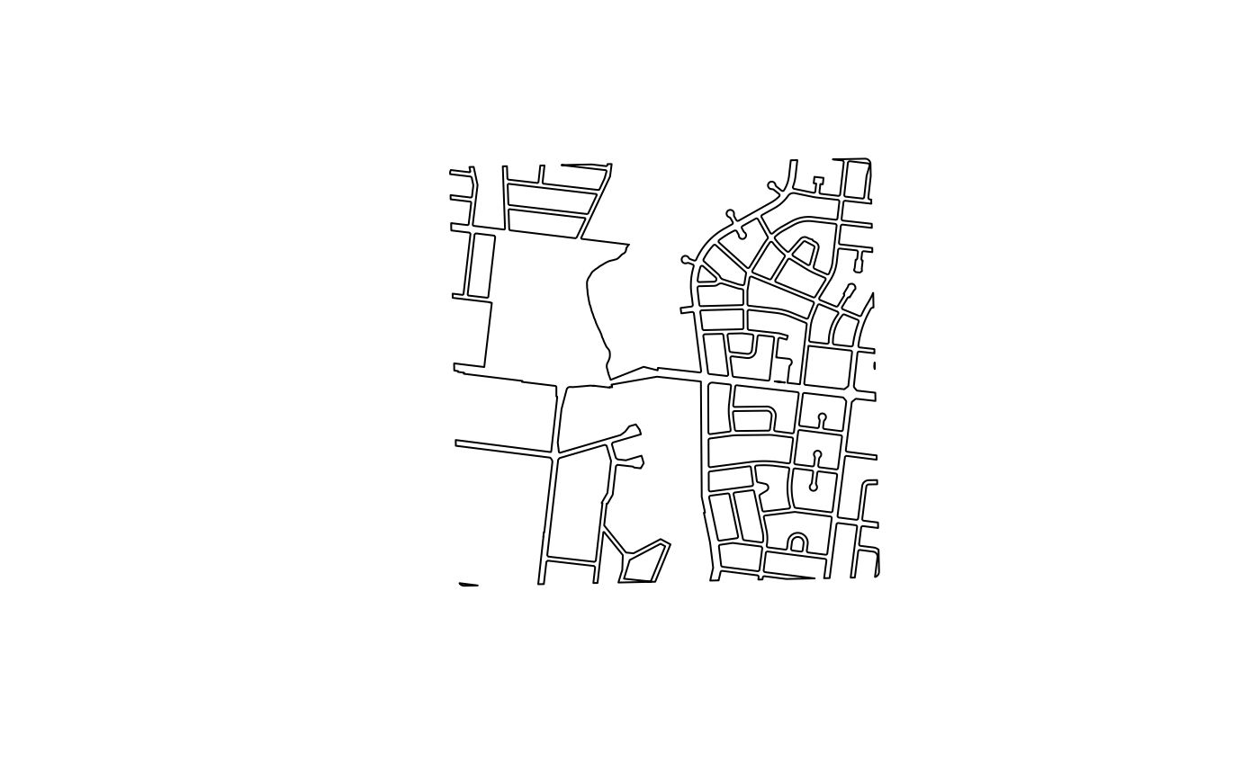
lizard_barrier_shp <- example_barrier_shp()
#> Reading layer `lizard_barrier' from data source
#> `/home/runner/work/_temp/Library/urbioconnect/ex/lizard_barrier.shp'
#> using driver `ESRI Shapefile'
#> Simple feature collection with 1 feature and 1 field
#> Geometry type: MULTIPOLYGON
#> Dimension: XY
#> Bounding box: xmin: 326089.6 ymin: 5820342 xmax: 327662.5 ymax: 5821909
#> Projected CRS: GDA94 / MGA zone 55
plot(lizard_barrier_shp)
# Load barrier shapefile
lizard_barrier_shp <- example_barrier_shp()
#> Reading layer `lizard_barrier' from data source
#> `/home/runner/work/_temp/Library/urbioconnect/ex/lizard_barrier.shp'
#> using driver `ESRI Shapefile'
#> Simple feature collection with 1 feature and 1 field
#> Geometry type: MULTIPOLYGON
#> Dimension: XY
#> Bounding box: xmin: 326089.6 ymin: 5820342 xmax: 327662.5 ymax: 5821909
#> Projected CRS: GDA94 / MGA zone 55
plot(lizard_barrier_shp)
 # Load barrier raster
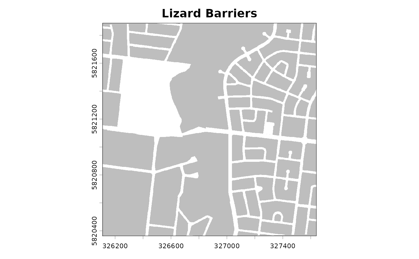
lizard_barrier <- example_barrier()
plot(lizard_barrier, col = c("grey", "white"), legend = FALSE, main = "Lizard Barriers")
# Load barrier raster
lizard_barrier <- example_barrier()
plot(lizard_barrier, col = c("grey", "white"), legend = FALSE, main = "Lizard Barriers")
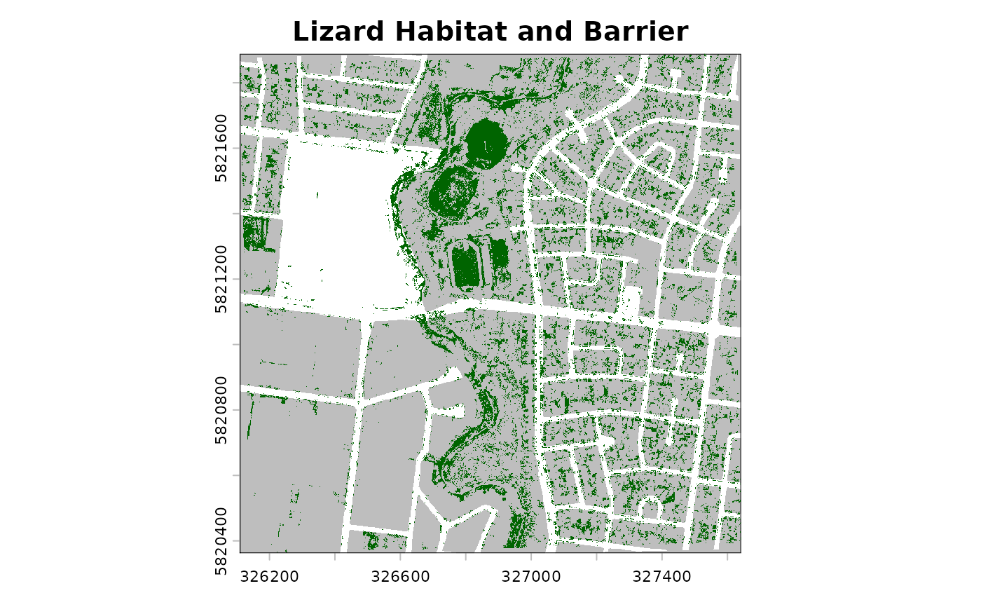
 plot(lizard_barrier, col = c("grey", "white"), legend = FALSE, main = "Lizard Habitat and Barrier")
plot(lizard_habitat, col = "darkgreen", legend = FALSE, add = TRUE)
plot(lizard_barrier, col = c("grey", "white"), legend = FALSE, main = "Lizard Habitat and Barrier")
plot(lizard_habitat, col = "darkgreen", legend = FALSE, add = TRUE)