Using raster vs vector • urbioconnect

library(urbioconnect)
library(terra)
#> terra 1.9.34
library(sf)
#> Linking to GEOS 3.12.1, GDAL 3.8.4, PROJ 9.4.0; sf_use_s2() is TRUE

urbioconnect can perform habitat connectivity analysis on either rasters from terra, and a vectors built on sf. Both implement the same underlying method from Kirk et al. (2023) and produce compatible outputs. The choice between them depends on your input data format and the scale of your analysis.

This vignette demonstrates the raster and vector methods on the same example data, compares their outputs, then offers practical guidance on which to choose.

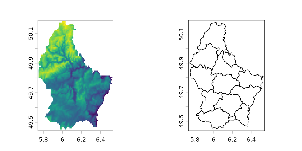
Rasters and vectors

Rasters are essentially matrices - grids of cells at a fixed resolution. Vectors are essentially polygons - shapes drawn by a line. See below an example of Luxembourg as a raster on the left, where the colour values correspond to elevation. On the right is a vector, showing the 12 different cantons.

urbioconnect uses rasters that work on SpatRaster (Spatial Raster) objects. Buffering is performed using a focal window (terra::focal()), and connected patches are identified using terra::patches().

The vector approach works on sf objects. Habitat and barriers are represented as polygons. Buffering uses sf::st_buffer(), and connectivity is determined by spatial intersection (sf::st_intersects()).

Both approaches expose convenience functions: habitat_connectivity() for rasters, and sf_habitat_connectivity() for vector. These run the full workflow in a single call.

Running raster and vector models on the same data

Prepare the example data

The package ships with lizard habitat and barrier data from Darebin Creek in Melbourne. The habitat is available as a raster, and the barrier as both a raster and a shapefile.

# Raster inputs
habitat_rast <- example_habitat()
barrier_rast <- example_barrier()

# Vector inputs
# Convert the habitat raster to polygons for the vector approach
habitat_sf <- terra::as.polygons(example_habitat(), dissolve = TRUE) |>
  sf::st_as_sf()

barrier_sf <- example_barrier_shp()
#> Reading layer `lizard_barrier' from data source 
#>   `/home/runner/work/_temp/Library/urbioconnect/ex/lizard_barrier.shp' 
#>   using driver `ESRI Shapefile'
#> Simple feature collection with 1 feature and 1 field
#> Geometry type: MULTIPOLYGON
#> Dimension:     XY
#> Bounding box:  xmin: 326089.6 ymin: 5820342 xmax: 327662.5 ymax: 5821909
#> Projected CRS: GDA94 / MGA zone 55

It is good practice to clean vector data before analysis, especially when working with real-world shapefiles that may contain topology errors or overlapping polygons. We have a clean() function in urbioconnect which runs sf::st_make_valid(), then unions the polygons, then simplifies with st_simplify().

barrier_sf_clean <- clean(barrier_sf)
habitat_sf_clean <- clean(habitat_sf)
interpatch_dist <- 10
buffered_radius <- interpatch_dist / 2

Raster approach

We will compare the raster and vector data timings, as well, using the tictoc package

library(tictoc)
#> 
#> Attaching package: 'tictoc'
#> The following objects are masked from 'package:terra':
#> 
#>     shift, size
tic()
raster_result <- habitat_connectivity(
  habitat = habitat_rast,
  barrier = barrier_rast,
  species = "Blue-tongued Lizard",
  interpatch_distance = interpatch_dist,
  verbose = FALSE
)
rast_time <- toc()
#> 2.686 sec elapsed

raster_result
#> # patch_connectivity:  data.frame
#> # Species:             Blue-tongued Lizard
#> # Patches:             703
#> # Resolution:          2x2
#> # Interpatch Distance: 10 m
#>   patch_id    area
#>      <dbl>   <dbl>
#> 1        1    60.0
#> 2        2  1648. 
#> 3        7    12.0
#> 4        8  1200. 
#> 5       10 92034. 
#> # ℹ 698 more rows

The raster result has columns patch_id, area (square metres), and area_squared.

Vector approach

tic()
vector_result <- sf_habitat_connectivity(
  habitat = habitat_sf_clean,
  barrier = barrier_sf_clean,
  species = "lizard",
  interpatch_distance = interpatch_dist
)
vect_time <- toc()
#> 10.34 sec elapsed

vector_result
#> # patch_connectivity:  data.frame
#> # Species:             lizard
#> # Patches:             483
#> # Resolution:          NA
#> # Interpatch Distance: 10 m
#>   patch_id  area
#>      <dbl> <dbl>
#> 1        1 1536.
#> 2        2  287.
#> 3        3  292.
#> 4        4  850.
#> 5        5    8 
#> # ℹ 478 more rows

The vector result has columns patch_id, area , and area_squared.

Comparing raster vs vector

Both approaches produce one row per connected habitat patch, with patch area and squared area.

nrow(raster_result)
#> [1] 703
nrow(vector_result)
#> [1] 483

Small differences in patch counts and areas are expected. The raster approach discretises space into cells, so patch boundaries are approximated at the chosen resolution. The vector approach preserves exact polygon geometry, so it typically produces slightly different (and arguably more precise) patch boundaries, particularly along curved or irregular barrier edges.

#> [1] 2.686

Timings for the methods are also important to consider. The raster approach took 2.686 seconds, and the vector approach took 10.34 seconds.

Summarising connectivity metrics

summarise_connectivity() works with output from either approach. You simply pass the appropriate area columns as vectors.

# Raster approach output uses the `area` column
summarise_connectivity(
  connectivity = raster_result$area,
  interpatch_distance = interpatch_dist,
  data_resolution = 10,
  species = "Blue-tongued Lizard (raster)"
)
#> # A tibble: 1 × 8
#>   species     interpatch_distance n_patches effective_mesh_ha prob_connectedness
#>   <chr>                     <dbl>     <int>             <dbl>              <dbl>
#> 1 Blue-tongu…                  10       703                 4           0.000015
#> # ℹ 3 more variables: patch_area_mean <dbl>, patch_area_total_ha <dbl>,
#> #   data_resolution <dbl>

# Vector approach output uses the `area` column
# Strip units before passing to summarise_connectivity
summarise_connectivity(
  connectivity = vector_result$area,
  interpatch_distance = interpatch_dist,
  data_resolution = NA,
  species = "Blue-tongued Lizard (vector)"
) 
#> # A tibble: 1 × 8
#>   species     interpatch_distance n_patches effective_mesh_ha prob_connectedness
#>   <chr>                     <dbl>     <int>             <dbl>              <dbl>
#> 1 Blue-tongu…                  10       483                 4           0.000016
#> # ℹ 3 more variables: patch_area_mean <dbl>, patch_area_total_ha <dbl>,
#> #   data_resolution <lgl>

The metrics — effective mesh size, probability of connectedness, mean patch area — will be close but not identical between the two approaches, reflecting the geometric differences described above.

Which approach should you use?

One factor to consider is what format your input data is already in. The other factor to consider is whether the data is large and computational time is important. For many situations, the raster based approaches will be much faster.

Situation	Recommended approach
Habitat data is a GeoTIFF or other raster	Raster (`habitat_connectivity()`)
Habitat data is a shapefile or GeoPackage	Vector (`sf_habitat_connectivity()`)
Very large study area (regional scale)	Raster (faster for large grids)
Small, precise study area	Vector (no resolution loss)
Need output maps or GeoTIFFs	Raster (native map output)
Exact polygon boundaries matter	Vector (no rasterisation artefacts)

Raster approach trade-offs

Faster for large study areas because operations run on regular grids
Straightforward to visualise as maps and export as GeoTIFFs for use in GIS software
Resolution must be chosen upfront: coarser resolution speeds up computation but loses fine-scale habitat detail
A slight loss of geometric precision is introduced when rasterising polygon inputs

Vector approach trade-offs

Preserves exact polygon geometry with no resolution-related approximation
Better suited to small, precisely delineated study areas
No need to choose a resolution
Can become slow for complex geometries with many vertices; running clean() beforehand helps

Converting between raster and vector

If your habitat is in raster format but you want to use the vector approach (or vice versa), conversion is straightforward.

# Raster to vector
habitat_sf <- terra::as.polygons(example_habitat(), dissolve = TRUE) |>
  sf::st_as_sf()

# Vector to raster (requires a template grid)
rasters <- prepare_rasters(
  habitat = habitat_sf,
  barrier = barrier_sf,
  data_resolution = 10,
  target_resolution = 500
)
habitat_rast <- rasters$habitat_raster
barrier_rast <- rasters$barrier_raster

prepare_rasters() handles the conversion from sf to SpatRaster at the resolutions you specify, aligning the habitat and barrier grids so they are ready for the raster approach.

Analysis step-by-step

Both approaches expose individual functions if you need finer control — for example, to inspect intermediate outputs or to substitute a custom step.

# Raster step-by-step
barrier_mask <- create_barrier_mask(barrier_rast)
remaining <- drop_habitat_under_barrier(habitat_rast, barrier_mask)
buffered <- habitat_buffer(remaining, interpatch_distance = 10)
fragmented <- fragment_habitat(buffered, barrier_mask)
patches <- assign_patches_to_fragments(remaining, fragmented) |>
  add_patch_area()
areas <- aggregate_connected_patches(patches)

# Vector step-by-step
buffered_sf <- sf_habitat_buffer(habitat_sf_clean, interpatch_distance = 10)
fragments_sf <- sf_fragment_habitat(buffered_sf, barrier_sf_clean)
remaining_sf <- sf_drop_habitat_under_barrier(habitat_sf_clean, barrier_sf_clean)
patches_sf <- sf_assign_patches_to_fragments(remaining_sf, fragments_sf) |>
  sf_add_patch_area()
areas_sf <- sf_aggregate_connected_patches(patches_sf)

References

Kirk, H., Soanes, K., Amati, M., Bekessy, S., Harrison, L., Parris, K., Ramalho, C., van de Ree, R., & Threlfall, C. (2023). Ecological connectivity as a planning tool for the conservation of wildlife in cities. MethodsX, 10, 101989. https://doi.org/10.1016/j.mex.2022.101989